MSc Thesis Defense · University of Amsterdam

Stable-edge filtering for passive device-class classification in OT networks under operational change

Jonathan van den Heuvel · supervisors dr. Chrysa Papagianni & dr. Cyril Hsu · KPMG Cyber: Max Kerkers, Eise Schild
Security & Network Engineering · 7 July 2026

One-line framing: a reproducible negative result, the mechanism behind it, and a constructive turn that locates the fix in the representation. State it plainly; neither bury nor oversell.

Operational Technology

You cannot scan a running plant.

Power grids, water plants, and factory floors run on devices that never stop talking. Probing them risks the process, so we identify each device by listening to its traffic instead.

The setting, told visually. Critical infrastructure runs on OT devices that constantly communicate; you cannot safely active-scan them, so passive traffic analysis is the pragmatic way to know what is on the network. The realistic question is robustness to operational change, not accuracy on a clean trace.

The idea under test

Real traffic is messy, so clean the graph first?

The problem. The traffic mixes stable links (an HMI polling a PLC) with transient ones: engineering sessions, maintenance, scans
What everyone assumes. Prior work deletes the transient edges "to improve precision", and takes for granted that this helps. Nobody has tested it

The hypothesis this talk falsifies "removing temporally non-persistent edges before classification yields better, and more change-robust, passive device-class classification than keeping them" As a filter: keep an edge only if it recurs in at least θ of the time windows. (W, θ) = (5 min, 0.8), fixed in advance.

The problem is the mixed graph; the assumption is that deleting transient edges helps (the closest prior work pre-filters "to improve precision"). The hypothesis is quoted exactly as the thesis states it. The stable-edge filter is how the hypothesis is operationalized.

The main question

Does deleting the non-persistent edges before classification improve OT device classification, and its robustness when the network changes?

0Baseline first, not a research question. On steady traffic the filter removes nothing, so it cannot help or hurt: this just fixes the reference point
RQ1Robustness: does the filter reduce the accuracy drop when a host's traffic changes?
RQ2Location: is the signal, and the harm, in a host's own features or its neighbours'?
RQ3A better way: can a protocol-aware representation restore robustness without deleting anything?

Open on the main question large; it shrinks to the top as the four rows reveal. The "0" row is the baseline calibration, deliberately not a research question (the filter is inert on steady traffic). Held-out hosts are devices never seen in training, one per class reserved each seed.

The testbed

A reproducible OT lab: a virtual bottling factory

20 hosts · 5 classes × 4
Modbus/TCP + S7
one passive tap, no scanning
4 change scenarios, edge-level ground truth
train on steady, judge on unseen hosts

Each class does a distinct job on the line; that job, and the traffic it generates, is what we classify.

The lab is a scripted bottling factory: four controllers drive the stages, supervisory stations watch, engineering workstations configure, historians log, IT gateways bridge out. 20 always-on hosts, 5 classes x 4. Ground truth is exact because every scenario is scripted. Train on steady state, judge on held-out hosts (host-level split, not window-level). 10 lab x 10 model seeds; five-class chance 0.20.

Setting the baseline

Before touching the filter: does the graph even help?

On normal traffic the filter removes nothing, so it cannot help or hurt here. This just fixes the reference point
Same six per-host features, two models: a graph neural network (GraphSAGE) and a plain, graph-free random forest
The random forest matches the graph model on unseen hosts (0.512 vs 0.490). So the graph adds no measurable benefit, and everything that follows holds for any classifier

faint bar = fit on training hosts · solid bar = accuracy on unseen hosts

The solid bars are equal: the graph buys nothing here.

Two setup checks on steady traffic: the filter is inert (removes zero edges), and the graph-free random forest matches the GNN on held-out hosts (0.512 vs 0.490, paired p = 0.037). So the graph adds no measurable benefit at this scale and the later results are classifier-independent.

RQ1 · robustness under change

The filter helps nowhere, and hurts the one real outage

0.448 → 0.358 Δ −0.089 · p = 0.027 · worse 8/10 seeds

Under maintenance, when a controller is actually paused. Neutral everywhere else.

Δ held-out macro-F1 (filtered − baseline), per scenario

Every bar at or below zero: it never improved robustness.

The headline. Four scenarios neutral (+0.000 / +0.000 / drift −0.020 non-significant p=0.500 / +0.004), maintenance significantly negative (Δ −0.089, p=0.027, 8/10). It removes 20 of 56 edges under maintenance, zero from steady state. Do not read weak-class per-class movements as signal.

Why maintenance breaks it

Delete a paused controller's polls, and it looks like an idle PC

1A controller is defined by the polls coming into it
2Pause it, those polls stop recurring, so the filter deletes them
3Its features collapse to all-zero: the model now reads it as an idle IT endpoint

That damage is in the host's own features (RQ2), so every classifier shares it, the graph-free forest included (−0.104).

the polls that define plc-1, deleted when it pauses · in-degree 20 → 0

The graph animation: the polls into plc-1 are deleted (they stop recurring during the pause), its feature vector collapses to all-zero, and it becomes indistinguishable from an idle IT endpoint. Exact, not statistical. Pooled controller recall 0.92 → 0.70; only the paused host's windows flip, so pooled F1 stays 0.82. RQ2: node-local features carry the signal (0.505) and the harm (both subsets −0.080 / −0.075).

Is the harm real, or an artefact?

Remove the same number of edges, four different ways

stable-edge (our filter): drop the least-repeating edges → hurts (−0.089)
random: drop the same number at random → harmless (+0.051)
byte-volume: drop the lowest-traffic edges → also hurts (−0.060)
phase-local (the ideal): drop only genuinely transient edges → removes nothing here

And the whole penalty lands on the one paused controller: −0.229, versus about −0.037 for the three that keep running.

maintenance Δ macro-F1 · same count removed, four rules

Only rules that strip the quiet polls hurt: it is which edges you delete, not how many.

The controls isolate the cause. Random removal is the key control: same count removed, no harm, so it is not that removing edges hurts. Byte-volume (a different content-blind proxy) reproduces the harm. Phase-local (the idealised filter) removes nothing. And leave-one-controller-out puts the whole effect on the paused plc-1 (−0.229 vs about −0.037).

RQ3 · a better approach

Three ways to fix it. Only one works.

Delete the "flaky" edgesthe stable-edge filter we just tested
✗ erases what defines the device
Add a temporal model to the same windowsa spatio-temporal GNN over the sequence
✗ the windows are flat, nothing to learn
Rebuild the windows from the protocol's messagescount the transactions each device sends per second
✓ each class has its own rhythm

The story: deletion failed (slides 7 to 9). Then the planned fix, a temporal model on the same 5-minute windows, is a pre-specified null (0.453 vs 0.413, p = 0.44) because those windows are flat for 95% of cells, an invertible recoding of the static aggregate. The suspect is the representation, not the model. The third approach changes what we measure.

RQ3 · the result

Measure the rhythm, and a simple model nails it

Same captures. Now each window just counts the messages each device sends per second. Every class has its own fixed rhythm
A plain random forest, trained on normal traffic only, gets every unseen host right: 1.000 under every change scenario. Even the fanciest model only ties it
But delete edges again, the same old filter on this better representation, and it breaks again: 1.000 → 0.793, for every model alike

held-out macro-F1 · old ceiling vs the rhythm representation vs the same, re-filtered

Deleting is the problem, not the representation.

Answers the "do we re-apply the old filter?" question directly: yes, and it re-creates the failure at full strength (Δ −0.207, p = 0.031), identically for every model, because it deletes upstream of them all. The rhythm: supervisory ~1 message/s, historian 0.5/s, engineering 0.2/s plus writes. A label-free clustering recovers the classes (ARI 0.31 → 0.78). The decisive variable is the representation, not the model.

Being honest about the 1.000

A mechanism, not a field number

The lab's rhythms are exactly constant by design, which is why the score is perfect. The field is jittered and overlapping, so there it would be a margin, not a certainty
So I stress-tested it: jitter the rhythms until classes overlap, and it still holds

0.956–1.000held-out on every scenario, jittered cadences, ten extra seeds

−0.163filter penalty fades to non-significant (p = 0.084)

each tick is one message · the three classes keep different rhythms even when jittered

The 1.000 reflects the lab's deterministic cadence design; in the field, polling is jittered, load-dependent, and overlapping, so separation would be a margin. Reported in the thesis (section 4.7.2): jitter the cadences and the pooled random forest still holds 0.956 to 1.000 held-out; the filter penalty weakens to −0.163, p = 0.084, no longer significant at the 0.05 level. Magnitude is also lab-specific (near-bipartite hub topology).

Contributions

A reproducible OT lab and four operational-change scenarios with edge-level ground truth, released with all code
An inductive, multi-seed evaluation, with controls, showing that content-agnostic edge filtering is fragile
A plain explanation of why the filter fails, and when its inverse can work
A controlled demonstration that the decisive variable is the representation, not the model

Future work

A harder cadence regime (heavier overlap, a non-hub topology) for the temporal-headroom question
A learned content-aware filter, trained on the lab's edge-level ground truth
Validation on a real, NDA-constrained OT trace
A window-length sweep, and the retrain-on-filtered control

Four contributions, as in the thesis: the artefact, the controlled negative result, the reason, and the demonstration of what actually matters. Negative plus mechanism plus constructive turn.

The conclusion, in one sentence

Deleting messy traffic to clean the graph throws away the very evidence that identifies a device, so the fix is a better representation, not a cleaner graph.

In practice: protocol-aware telemetry first, aggregation second, content-agnostic deletion not at all.
Jonathan van den Heuvel · University of Amsterdam · 7 July 2026 · Thank you. Questions?

Lead with the human sentence; the practitioner ordering (telemetry first, aggregation second, deletion not at all) is the thesis's own closing line, kept small. Backup slides follow: type #16 to #28 in the URL bar, or arrow onward.

Backup

Backup slides, for questions.

16 the baseline · 17 graph utility · 18 the model ladder · 19 why 1.000 is not leakage · 20 jitter · 21 per-class · 22 the control table · 23 the confusion matrix · 24 θ and scope · 25 distribution shift · 26 external validity · 27 the content-aware filter · 28 the literature

Jump by editing the URL hash (#16 to #28) or arrow past this slide. Number keys 1 to 9 cover the main arc only.

Backup · the question scheme

Why the steady-state baseline is not a research question

The filter removes zero edges from a stationary phase, so filtered and unfiltered are identical by construction
A comparison the filter can neither win nor lose proves setup validity, not a hypothesis
What it calibrates: the held-out ceiling (0.490) that the change scenarios are judged against, and the graph-versus-no-graph reference
The thesis says it plainly: "This is a validation step, not a research question."

The question scheme puts the substance first: robustness under change is RQ1 because that is where the filter can actually act, and where the hypothesis says it should help. Steady state is the floor the rest stands on.

Numbered research questions carry hypotheses; the steady-state baseline is labelled calibration because the filter is inert there by construction. It fixes the 0.490 held-out ceiling and the graph-versus-no-graph reference.

Backup · graph utility

"Why a graph thesis if the graph adds nothing?"

RF 0.512 vs GraphSAGE 0.490 on held-out hosts: mean difference +0.022, 95% CI [+0.004, +0.049], paired p = 0.037
Treated as a result: at 20 hosts and six features, message passing adds variance faster than signal
The maintenance penalty reproduces in the random forest (−0.104), so the finding is feature destruction, not a message-passing artefact
That makes every conclusion hold for any classifier reading the features, which is more robust, not less

held-out macro-F1, random forest vs GraphSAGE

The graph is inert at this lab's scale (20 hosts, six features) and the thesis treats that as a result; whether message passing helps at larger scale is explicitly left open, and every conclusion holds for a graph-free classifier.

Backup · the model ladder

Five models, one identical collapse

On the cadence representation every rung reaches the ceiling: RF pool, GRU no-graph, GNN mean-pool, static GraphSAGE, temporal GNN
The temporal GNN dips to 0.973 on two scenarios, from a single unstable seed
Filtered input: all five land on 0.793, identically; the damage is upstream of every model
One caveat the thesis states itself: the five per-model tests share identical per-seed numbers, so this is one result, not five confirmations

maintenance, held-out macro-F1 · unfiltered vs stable-edge-filtered, per model

Temporal capacity adds nothing once the windows are informative, and recovers nothing once the filter has deleted the signal. The representation sets the ceiling and the floor.

Backup · the perfect score

Why 1.000 is not overfitting or leakage

Trained on steady state only; scored on hosts never seen in training
Survives protocol changes: the secondary leave-one-scenario-out protocol reproduces 1.000, and the same 0.793 filtered penalty
Not carried by the easy fifth class, and not by pooling
The same pipeline visibly can fail: the filter drops it to 0.793, which a leak would mask
And the score has a cause you can inspect: class-constant cadences, separable in a single window

0.957–1.000per-window scoring, no pooling at all

1.000four-class macro-F1 excluding the IT class (0.97 per window)

0.31 → 0.78label-free clustering recovers the classes (Adjusted Rand Index)

−0.207the same pipeline shows the filter's full failure mode

The honest scope stays: the perfection reflects the lab's deterministic cadences. The claim is the mechanism; the jitter sweep (slide 20) is the falsification test of that claim.

Backup · non-constant cadence

The jitter sweep: the finding survives realistic cadences

Ten extra lab seeds with jittered, overlapping per-class poll intervals, redrawn per run
Pooled RF, still trained on steady state alone: 0.956 to 1.000 held-out on all five scenarios
The maintenance margin narrows exactly where predicted: 1.000 → 0.956
The filter penalty is directionally preserved but weaker: Δ −0.163, worse 6/10 seeds, p = 0.084, no longer significant at the 0.05 level
Still open, stated as such: whether temporal capacity helps when margins are genuinely thin needs a harder regime

held-out macro-F1 per scenario, pooled RF, train-on-steady · dashed line = chance 0.20

Reported in the thesis as non-significant rather than claimed. Both margins narrow without overturning the representation finding: the separability is a property of the representation, not of exactly-constant intervals.

Backup · per-class reality

Per-class reality: the macro is carried by controller and IT

Steady state · held-out F1 per class

class	F1
controller	1.00
IT endpoint	1.00
engineering	0.24
supervisory	0.12
historian	0.10

The three middle classes form a three-way confusion (three-class macro 0.15; four-class, excluding IT, 0.36). The mechanism findings live in the well-resolved controller class.

Maintenance · baseline → filtered

class	base	filt	Δ
controller	0.96	0.82	−0.13
supervisory	0.10	0.00	−0.10
engineering	0.23	0.38	+0.15
historian	0.13	0.14	+0.01
IT endpoint	0.90	0.71	−0.19

Engineering improves and historians are unchanged, as the thesis's own table caption notes; it builds no mechanism claim on the weak-class movements. The damage lands on the classes the model actually resolves.

0.490 is about 2.4 times the five-class chance level of 0.20, carried by controller and IT; the three middle classes are near-unresolved at this scale, which the thesis states. The cadence representation later resolves all five.

Backup · the numbers

Maintenance Δ by selection rule

All 10 lab × 10 model seeds, paired Wilcoxon. Same count of edges removed per window; only rules that target the low-volume polls are harmful.

Leave-one-controller-out concentrates it: paused plc-1 −0.229 (p = 0.002, 10/10) vs −0.040, −0.040, −0.031 for the running three.

stable-edge (persistence) −0.089p = 0.027 · worse 8/10 · the thesis filter
byte-volume −0.060p = 0.004 · worse 9/10 · also harmful
random count-matched +0.051p = 0.160 · worse 3/10 · harmless, rules out "any removal hurts"
phase-local 0.000removes nothing by construction · the penalty is the observation window
content-aware +0.000keeps the control-port polls, still prunes scanners (slide 27)

The contrast between random (harmless) and persistence / byte-volume (harmful) is the heart of the controls: which edges are removed, not how many.

Backup · the misclassification

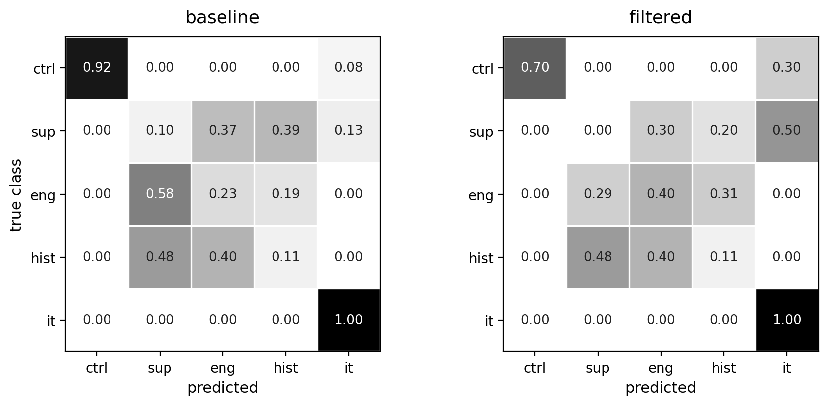
Filtering shifts the paused controller toward "IT endpoint"

Controller recall falls 0.92 → 0.70
The controller-to-IT cell rises 0.08 → 0.30: the leak is specifically toward the idle-endpoint signature
High precision keeps controller F1 at 0.82, not zero; supervisory windows are pushed the same way, toward the idle-IT signature

maintenance confusion matrices, baseline vs filtered

Recall (0.70) and per-class F1 (0.82) reconcile because the 0.30 is the leak, not the recall. The direction of the leak, toward the idle-IT signature, is the mechanism made visible.

Backup · operating point

Harmful at every θ that removes edges, and a closed-form scope

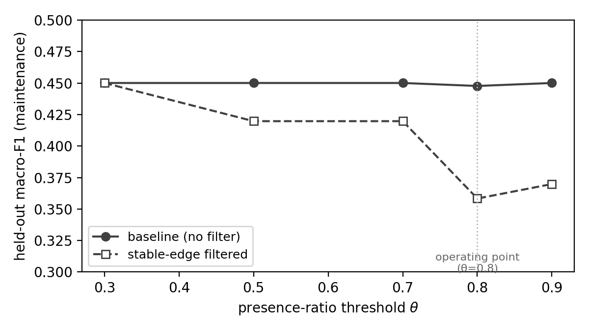
θ swept 0.3 to 0.9 at W = 5 min: 0 edges removed at 0.3, 10 at 0.5 to 0.7, all 20 at θ ≥ 0.8
Δ runs from −0.030 (θ = 0.5) to −0.089 (θ = 0.8); beneficial at none
Scope condition: removal is guaranteed when the interruption exceeds the 1−θ fraction of the horizon; here 0.27 > 0.2
Shorter captures, longer outages, or recurring maintenance keep a deployment inside the harm regime; longer observation (Heo and Shin's remedy) moves it out

maintenance macro-F1 versus presence threshold theta

The sweep shows harm at every θ that removes edges. The scope condition bounds the harm regime in both directions; a passive operator at a single tap cannot know which side of the 1−θ boundary they are on. The window-length W sweep is future work.

Backup · distribution shift

"Isn't it just train-dense / test-sparse shift?"

The filtered model trains on dense steady-state graphs and tests on sparse filtered ones, so the objection is fair
Control: train on randomly-sparsified steady-state graphs, then test on filtered maintenance
The penalty persists: Δ −0.126, p = 0.006. Not pure covariate shift
The count-matched random removal argues the same way: equal test-time density, no harm
A direct retrain-on-filtered control would settle it completely, and is stated future work

Two controls point the same way; one is deliberately left open, and the thesis does not over-claim closure. This is the cleanest alternative explanation, met with the strongest available evidence and an honest residual.

The randomly-sparsified-training control (−0.126, p = 0.006) and the count-matched random control argue against pure covariate shift; the retrain-on-filtered control is stated future work, and the thesis does not claim the question is fully closed.

Backup · external validity

"n = 1 lab, n = 1 paused controller, isn't the failure engineered?"

The magnitude is lab-specific, conceded: the near-bipartite poll topology means a paused PLC here loses essentially its whole footprint
A field PLC keeps peer, historian, and management traffic: partial collapse, smaller penalty
The mechanism is the claim, and a second proxy (byte-volume) reproduces it: proxy-generality, not yet topology-generality
A second, non-hub topology is named as the first test; field validation on a real trace follows

The split between magnitude (concede) and mechanism (defend) is stated in the thesis itself, in the threats-to-validity section, together with the boundary of what does not transfer.

The thesis's threats-to-validity section separates magnitude (lab-specific, near-bipartite hub topology) from mechanism (reproduced by the byte-volume proxy); a non-hub topology and a field trace are the stated next tests.

Backup · the selection-layer fix

A content-aware filter removes the failure mode

Rule: keep any edge addressed to a control-protocol port (Modbus/TCP 502, S7 102, and analogous), regardless of persistence; apply the persistence test only to the rest
Under maintenance it removes no edges: Δ +0.000, against −0.089
Under benign noise it still prunes the eight scanner edges (about 1.6 per window), all on non-control ports: selective, not disabled
The crudest form of content-awareness; the principled successor is a learned edge filter, trained on the lab's edge labels

−0.089 → +0.000 maintenance Δ · content-agnostic → content-aware Where deletion is wanted at all, the rule must read edge content, not a structural proxy. Safe where the content-agnostic filter is harmful, while keeping its pruning behaviour elsewhere.

Honest framing: it removes a failure mode, it does not raise accuracy (the graph is inert at this scale). The representation result on slide 11 is the deeper fix; this is the selection-layer one.

Backup · positioning

What the closest prior work does, and does not, test

Heo and Shin (2025): pre-clean the graph "to improve precision"; robustness = added attacker hosts and packet noise; remedy = longer observation
Brown et al.: random edge removal degrades gracefully; separately, accuracy decreases as synthetic links are added
In all prior work the pruning is incidental, its classification effect never isolated
"None treats temporal persistence ... as the filter." This thesis tests exactly that, under four scripted changes

work	robustness eval	reprod.
Heo and Shin	attacker hosts, noise	partial
Brown et al.	edge removal	data
this thesis	operational change (4)	yes

Method note: Heo and Shin cluster byte-sequence images over a static graph, with no temporal or graph-neural model; this thesis is a test of their implicit preprocessing assumption, not a reproduction of their system.

Attribution discipline: the accuracy-decreases-when-links-are-added finding is Brown et al., not Heo and Shin. Heo and Shin's robustness axis is added hosts and packet noise.